
There are two ribbons dedicated to profile windows, General and Analyze, which is described below. The availability of the various functions will depend on whether the curves are shown in Analysis View or Comparison View mode.


When the Select tool is highlighted none of the other tools are active. When clicking one of the drawing tools the active tool will be highlighted while the Select tool will be shown normally until the use of the drawing tool has finished. During drawing the mouse cursor will be seen as a shape reflecting the chosen tool instead of the normal mouse arrow.
You can zoom in a profile window when it is shown in Analyze view by:
To turn off zooming, click Zoom > 100% or the Home key.
When zoomed, the lower right corner of the window will have transparent icon indicating that the profile is zoomed and that not all points are visible. Below is a profile window shown before and after zooming into a peak.
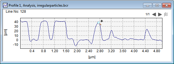
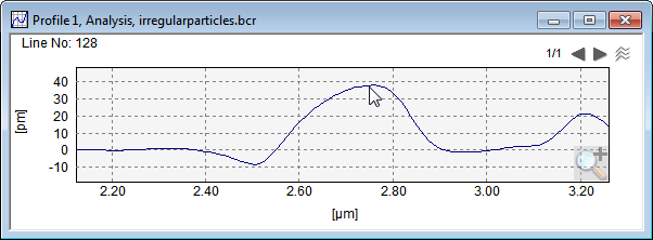
When the panning tool is selected the zoom area can be panned either by dragging any position in the drawing area of the profile window
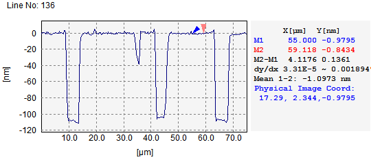
Cursors for measuring for example height and length differences can be turned on pair wise.
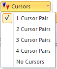

When cursors are turned on the cursor positions and their differences will be written in the right part of the profile window. You may also change the number of cursor pairs incrementally by clicking the 'C' on the keyboard.
The Inspection Box allows you to inspect a specific part of a curve by drawing a box around the region of interest and have this part shown in its own profile window, see below:
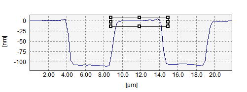
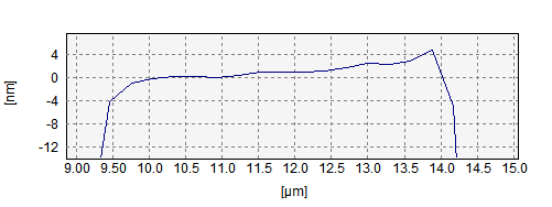
The Inspection box may also be used for limiting the fitting range (both in x and y) for polynomial fit,

This function is used for indicating the height and length differences of the cursors. The written values correspond to the "M2-M1" values shown in the table to the right.
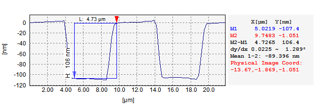
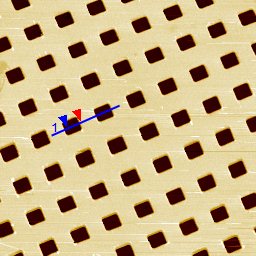
This option will visualize the profile cursors in the parent image window at their corresponding positions:
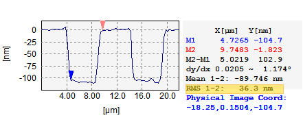
When Show RMS is on the RMS value of the profile between the cursors will be reported in the right table.

In Auto Scale Mode the range of the y- and x-axes will be set to give a good usage of the plot area, with only little space at the top and bottom and no space left and right.
Setting Freeze Axes will freeze the y- and x-axes to their current range, such that a change of the profile(s) (for example by moving the profile line in the source image window) will be reflected on the same scale. This serves as a good facility for comparing profiles on the same scale.
Setting Aspect 1:1 will set the aspect ratio to 1:1 so that the x, y ratio will appear geometrically correct. Note, that many profiles are extremely flat and may therefore in this mode appear close to a straight line.
The Range field allows you to browse through a number of predefined y-ranges following a 1, 2, 4, 10 , 20 .... sequence system. This makes it easy for you compare different curves on the same scale.
This will activate the Graph Property dialog for the selected curve where more curve properties can be set.
Click the Dialog Box Launcher to open the View Settings Pane.


The Leveling pull down menu contains predefined leveling settings for profiles that will be applied when selected:
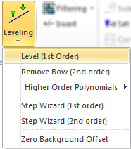
In Analysis View mode only the shown curve will be leveled where as the entire curve set will be leveled when shown in Comparison View mode.
You can use a number for predefined built-in or customized filters by selecting them from the Filter Quick Launch pull down menu:
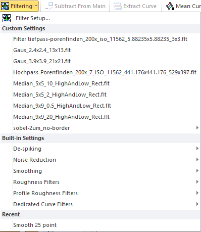
Click Filter Setup to open the Filter Dialog where you interactively can construct various filter type, for example, for smoothing, noise removal or as a preprocess for roughness calculation.
In Analysis View mode only the shown curve will be filtered where as the entire curve set will be filtered when shown in Comparison View mode.
The Invert function will multiply the selected profile Y-values by -1.0. In Comparison View all profiles will be inverted while only the selected curve will be inverted in Analysis View.

Subtract from Main will subtract the current profile from all horizontal profiles in the Main Image window. This may be a good tool for removal of a repeated structure or noise. It is required that the number of profile points equals the number horizontal points of the main image.
The source image of the profile can be offset so that y-value at the active cursor position is subtracted from the entire image. This is equivalent to offsetting the image such that the active cursor point is set to zero.
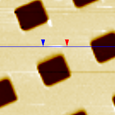
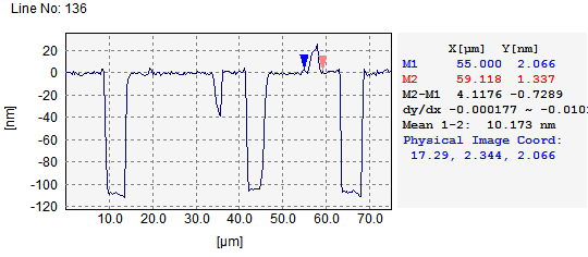
The Correct Scan Line tool is used for correcting entire scan lines or part of a scan line, which for example suffers from contamination or noise artifacts. The correction will be performed on the source image, thus it is required that the profile has a parent image window and that it is set horizontally.
If the cursors are active only the part between the first cursor pair will be corrected.
The correction will be performed by three optional techniques:

|
|

|
|
Image and profile pair before and after correction of profile piece between cursors.
This panel is dedicated to function only available when the profile window is in the Comparison View mode and will be described in the Cross-Section Profiling Comparison View section.
The analytical functions related to profile windows are found in their Analyze Ribbon and the panels with their functions are described below.


When clicking this button the Roughness Analysis Pane will be opened and the active profile window will be defined as the source window for roughness analysis. Before performing the calculation you should assure at the various settings at setup appropriately in the Roughness Analysis Pane. The analysis will be performed on the entire set.
You can learn more about roughness in the Roughness Analysis section.
You can get at the histogram calculated and seen in a Histogram Window with dedicated functions.The histogram will stay on until you turn it off again or close the histogram window. While on it will be updated automatically whenever the profile is modified likewise it be updated when browsing through a collection of curves.
You may calculate the Fourier transform (amplitude) by a Fast Fourier Transform (FFT) algorithm with normal resolution where the number of Fourier points equals the number of points in the profile. Alternatively you can get the Fourier transform calculated with extended resolution ( x 16) where the number of Fourier points is 16 times larger (by use of mean value padding). Please note that in a 1D Fourier window only the right half of the Fourier transform is seen because it is a redundant mirror of the left part.
Like the Histogram window the Fourier window will be updated when the profile is modified or when browsing through a collection of curves.
Click this button to activate the ISO 5436 Step Height dialog for calculation of the step height. The calculation will be updated whenever the profile is being modified or when browsing through a set of curves. Likewise the connected Step Height result grid will be kept updated.
To calculate the first order derivative (dy/dx) click the Gradient button.
Like the Histogram window the Gradient window will be updated when the profile is modified or when browsing through a collection of curves.
Click this button for activating the Calculator Pane where you can perform mathematical operations using entire images or profiles.

This panel contains functions for fitting polynomial functions and subtract fit results from the profile data.
A polynomial fit from zero to 9th order can be activated by this "split button". When active the polynomial fit will be shown together with the profile data.
The fit range (both in x and y) can be limited by the Inspection Box.
Click Subtract Now to subtract the fitted curve from the profile data.
Subtract the fitted curve whenever the profile is modified.

Click this button to get at Square Wave fit to the curve, see the section about Quadrangle Fit
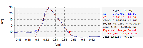
You may turn on the Cone Angle Fit and have it shown and reported as shown below. When the cursors are on the cone angle will be fitted to the curve piece between the first cursor pair, otherwise the entire curve will be fitted.
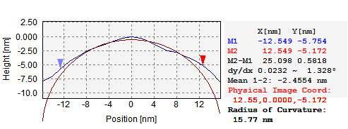
Turn Radius of Curvature on to have it shown and reported
When right clicking in the Profile window a context menu will appear:
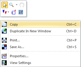
The context menu will have a "Floaty" section at the top with small icon buttons by which you can access the common tools for working with profiles described previously.
Below is a more traditional menu with generic functions typically available for all data windows. One menu item is the Properties, which is described below.
The Property dialog provides more detailed control of the functionality of the graphs.
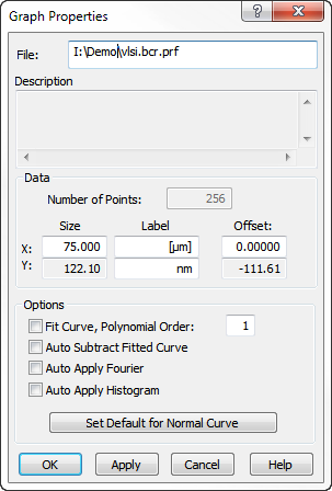
The default parameters will be stored along with their associated curve types, such that the default settings for, e.g., Fourier graphs are independent from the other curve classes.
By use of the right mouse popup menu or CTRL+C is possible to copy the window content to the Clipboard of the operating system from where it can be pasted into, for example, word processors. It is also possible to print the window or save it to an ASCII file or the STM-BCR file format or save the graphics in one of the supported graphics formats.
The ASCII file contains the floating point x, y co-ordinate and can be imported by, for example, spreadsheet programs while the STM-BCR format is recommended for usage in SPIPTM.
When more profiles are desired for comparison it is possible to keep a copy of any profile by the Duplicate menu item.